[Python] LSTM을 이용한 주가 예측

LSTM의 구조 및 특징

1. RNN에 비해 무한대의 기억 능력

2. RNN의 gradient 문제 극복

3. Momory Block 구조

     - sigmoid 함수 계열의 activation function이 사용됨 (hard sigmoid를 사용하면 성능 UP)

     - output을 만들 때는 tanh 함수 사용

LSTM 기반 주가 예측

  - 주가는 정상성을 만족하지 않음

  - 수익률 자체도 정상성을 만족하지는 않음 ( ← 수익률 평균이 일정하지 않으므로)

      ⇒ 비정상성 제거 후 예측 진행

  - EMA(Exponential Moving Average) 이용

import yfinance as yf
import pandas as pd
import numpy as np
import talib

# 데이터 다운로드
start = '2017-12-16'
end   = '2022-12-15'
KOSPI  = yf.download('^KS11', start, end) #KOSPI index

보통 6년치 데이터 다운로드 받음 (train : 5년, test : 1년)

 

KOSPI.head()

 

shape은 (1226, 6)

 

# 조정 종가 사용
kospi = KOSPI['Adj Close']

# 수익률과 비슷한 데이터 생성
kospi = np.log(kospi) - np.log(talib.EMA(kospi, 10))

10일치 EMA를 통해 최근 지수를 반영한다.

 

from statsmodels.graphics.tsaplots import plot_pacf

plot_pacf(yt, lags=40, method='ols', title='Partial Autocorrelation').show

 

 

하늘색으로 색칠된 부분은 신뢰구간

p = 3 일 때 구간 밖으로 나와있음 (뒤에 몇개 구간 밖에 것들은 노이즈로 취급)

→  p = 3으로 결정

 

yt_1 = yt.shift(1) # 1일 전 adjusted kospi
yt_2 = yt.shift(2) # 2일 전 adjusted kospi
yt_3 = yt.shift(3) # 3일 전 adjusted kospi

data = pd.concat([yt, yt_1,yt_2,yt_3], axis=1)
data.columns = ['yt', 'yt_1', 'yt_2', 'yt_3']
data = data.dropna()
data.head()

 

# 주가 예측을 위한 종속변수 및 독립변수 지정
y = data[['yt']]
x = data[['yt_1', 'yt_2', 'yt_3']]

#pip install sklearn
#!pip install scikit-learn

from sklearn import preprocessing

num_attrib =3
scaler_x = preprocessing.MinMaxScaler(feature_range = (-1, 1))
x = np.array(x).reshape((len(x), num_attrib))
x = scaler_x.fit_transform(x)

num_response = 1
scaler_y = preprocessing.MinMaxScaler(feature_range = (-1 , 1))
y = np.array(y).reshape((len(y), num_response))
y = scaler_y.fit_transform(y)

# train : 전체 데이터의 80%, test : 20% 
train_end = int((x.shape[0]*0.8))

x_train = x[0:train_end, ]
x_test  = x[train_end:data_end, ]
y_train = y[0:train_end]
y_test  = y[train_end:data_end]

# 2차원 -> 3차원으로 reshape for LSTM
x_train = x_train.reshape(x_train.shape[0], 1, x_train.shape [1])
x_test  = x_test.reshape(x_test.shape[0] , 1, x_test.shape [1])

print(" Shape of x_train is ", x_train.shape)
print(" Shape of x_test is ", x_test.shape)

#!pip install keras
#!pip install tensorflow

from keras.models import Sequential
from keras.layers.core import Dense, Activation
from keras.layers import LSTM
#from keras.layers.recurrent import LSTM

seed = 2016
np.random.seed (seed)

fit1 = Sequential()
fit1.add(LSTM(units = 4, # 수정가능
              activation = 'tanh',
              recurrent_activation = 'hard_sigmoid',
              input_shape =(1, 3)
             )
        )
fit1.add(Dense(units = 1, activation = 'linear'))

fit1.compile (loss ="mean_squared_error", optimizer ="rmsprop")  # Root Mean Sqaure Propagation

fit1.fit(x_train, y_train, batch_size =1, epochs =10, shuffle = True)

print(fit1.summary())

 

학습 결과

• 시계열 데이터를 3단위로 잘라 input으로 넣음
• 훈련이 3단위로 이루어짐 : 각 단위 내에서는 시계열로 이루어져있음
• shuffle을 해도 문제 없음, 성능이 더 높아짐

score_train = fit1.evaluate(x_train, y_train, batch_size =1)
score_test  = fit1.evaluate(x_test, y_test , batch_size =1)

print ("in train MSE = ", round(score_train, 4))
print ("in test MSE = ", round(score_test, 4))

train MSE : 0.0064

test MSE : 0.0063

=> MSE 가 아주 작음

 

pred=fit1.predict(x_test)
pred1=scaler_y.inverse_transform(np.array(pred).reshape((len(pred),1)))
y_test1=scaler_y.inverse_transform(np.array(y_test).reshape((len(y_test),1)))

%matplotlib inline
import matplotlib.pyplot as plt

plt.plot(y_test1, marker = '^', label = "Original series")
plt.plot(pred1, marker = 'o', label = "Prediction")
plt.legend()

 

추세가 비슷함

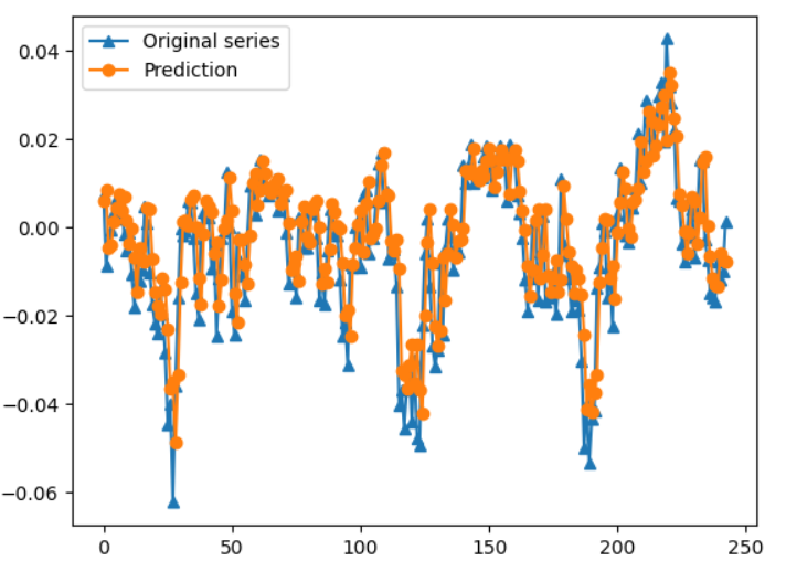
두 그래프가 거의 유사 : 예측 성공

 

 

 

 

---

본 자료는 중앙대학교 블랙스톤 금융AI 아카데미 (Blackstone Financial AI Academy) 코딩 부트 캠프 강의 자료를 참고하여 제작하였습니다.